Lossy and Lossless Compression

Compression is a means to convey the original information with fewer bits/pixels, so that the storage and transfer of information can be more efficient.

In lossy compression, some of the data in the original file is removed to save space, which is what we as humans recognise least, so there is without any noticeable difference from the original file after compression. For example, ultrasonic frequency in the music recording will be ignored as humans cannot hear this band of frequency. On the other hand, humans are very sensitive to frequencies in the vocal range, so it is wise to preserve the quality at this range as much as possible. In the extreme case, humans can hear deep bass, but we’re less attuned to it. Therefore, lossy audio compressors encode different frequency bands at different precisions by taking advantage of this, of which humans cannot distinguish the difference.

However, in some occasions, the audio compression is so prominent that we perceive different sound quality on a cell phone versus in person, which is for the sake of allowing more people to take calls at once. As more and more data is removed from the compression algorithm, the signal quality or bandwidth would be deteriorated.

The format commonly used lossy compression algorithms are JPEG, MP3, and MPEG-4, correspondingly the file extensions are .jpg, .mp3, .mp4. The compression reduces certain precision in a way that aligns with human perception is called perceptual coding from the field of study called psychophysics. Humans are good at detecting sharp contrasts, such as the edges of objects, but subtle colour variation is remarkable to human perception.

Taking JPEG as an example, which stands for Joint Photographic Experts Group. Image can be represented by a matrix, an element with the higher value means brighter, vice versa. Storing each of the values in one byte can give us a range of 0 to 255 for each colour. Colour images have different channels for each colour component, which becomes a 3-D array. However, it is inapplicable. Say we have 3,000px x 4,000px, then we have in total 3000x4000x3=36,000,000 px. For storing them as 8-bit integers, we should have 36MB file size. By using JPEG image compression, the file size becomes 1.83MB.

This can be done by the following steps. Colour Space Conversion is to convert the RGB channel into colour space, i.e. YCbCr, where Y represents the light intensity while the CbCr represents the colours. This linear transformation can be expressed as a matrix multiplication, which provides a separation of the luminance from the chrominance components that our visual system favour change in brightness than colour. This process is called chroma subsampling, which is widely used in image and video processing pipelines. Besides, as humans are prone to ignore small objects or fine details in a picture as compared to the large ones, we can also take advantage of the frequency-dependent contrast sensitivity.

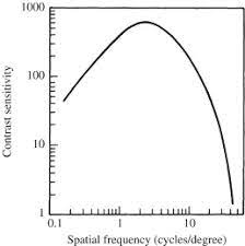
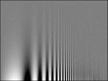
The spatial frequency of the bars increase from left to right and the contrast decreases from the bottom to top. The bars under the curve are more visible than the rest. We are more sensitive to brightness variation in this range of spatial frequencies. At the upper right hand corner, though there are some many subtle differences among pixels, humans cannot register all those details, this should be the area for compression.

Images can be compressed by dividing the image into 8x8 blocks and quantise them in a frequency domain representation. This maintains the visual essence, but might only use 10% of the data. Comparing the 8x8 blocks with 64 frequency patterns which decompose the image into its frequency components, converting an 8x8 block where each element represents a brightness level into another 8x8 block where element represents the presence of a particular frequency component. This process is called Discrete Cosine Transform (DCT). So, we can easily compress the frequencies that are less visible to human beings by dividing these frequency components with some constant and then quanitse them. These components are divided by larger constants as compared to the ones that we are more sensitive to, and then round them to the nearest integers. As a result, most of the values shrink to zero. It definitely enhances the compression rates but it also lowers the image quality. We can store the information more efficiently by re-arranging the elements in a zig-zag order from top left to bottom right into an array.

Video compression is very similar to the lossy image compression, it even further compressed the unchanged steady background by temporal redundancy. Those pixels that appear every frame in the video should not be re-transmit, patches of data will be copied instead. By taking advantage of inter-frame similarity, it is more efficient to transmit only the small pixel differences. These methods can be applied to rotation, brightness, translation, etc. MPEG-4 is a common standard compression format that is 20 to 200 times smaller than the original file. Encoding frames can cause distortion when the compression is too heavy or there is not enough space to update pixel data inside the patches.

However, the compression is less commonly used with text, as it is very noticeable with the missing data. Nonetheless, it depends on the usage, if we compress the image, we may see the edges of the object that may not be preferable to visual arts. So before compression, we should weigh between quality and saving space.

In lossless compression, no data is removed but it’s rearranged so that the redundant data can be stored efficiently. WAV and FLAC provide uncompressed audio format. For the number of zero we have in the array, we can store the number of times they consecutively occur in tuples, which is called run length encoding (RLE). RLE can replace the repeated data, i.e. runs with frequency/data pairs. It works best with data likely to have lots of repeats. The longer the runs, the more efficient is the compression, vice versa. The arrangement can be easily expanded to the original form without any degradation, so the decompressed data is identical to the original before compression, bit for bit.

We can further compress what’s left by encoding the more frequent values with fewer bits and less frequent values with more bits so that we can reduce the average number of bits per symbol. This more compact algorithm that is like converting “Don’t forget to be awesome” to DFTBA, a dictionary is needed to store the mapping from codes to data. In this representation, string does not seem as a string of individual pixels, but as blocks of data. For example, there are 4 pairings in the blocks of data: White-White, White-Black, Black-White, Black-Black. These are the data blocks in the dictionary for which compact codes are generated. It is common that all these blocks would occur at different frequencies, like 4 WW, 2 WB, 1 BW, and 1 BB. WW is the most common block which will be substituted for the most compact representation, while 1BW and 1BB can be substituted for something longer because those blocks are infrequent.

Considering the following text:

"ABRACADABRAABRACADABRA"

What we need to do firstly is to scan the text to be compressed and count the occurrence of all characters. the priority list and the character are sorted according to frequency in ascending order. Secondly, the lowest frequency nodes are chosen to be co-joined with one node and add their frequency to be the frequency of the new node. By joining SP and period, the new node has the frequency 2. Thirdly,

A us coded with 0, SP is coded as 1000, period is coded with 1001, B is coded with 101, R is coded with 110, D is coded with 1111. So each letter in the coded word is replaced by its code.

The letter with the highest frequency is replaced with shortest code. From the table, A with the highest frequency (10) is coded by one bit which is 0, while the letter with the least frequency like SP and period are both coded with 4 bits, 1000 and 1001 respectively.

This generating efficient codes method is to build a Huffman Tree, which is called Huffman entropy coding. This algorithm is processed that firstly all possible blocks and their frequencies will be layout, then two blocks with the lowest frequencies will be selected. In the above example, BW and BB will be grouped, then it is with WB, finally all these will be combined with WW. Therefore, it is observed that the groups arranged by frequency will deliver a tree like pattern. To put this frequency-sorted tree into a dictionary, labelling each branch with a 0 or a 1 can generate the code. 0 for WW, 10, WB, 110 for BW and finally 111 for BB. As each path down the tree is unique, there is no conflict among branches, which contributes to prefix-free (no code starts with another complete code). Ultimately, 10-110-0-0-0-111-10-0 will cost 14 bits of data representing the order of arrangement. This will be appended in the way of 10110000-111100 to the front of the image data , including the dictionary, which costs 30 bytes rather than 48 bytes in the original data. These two compression algorithms are implemented in PNG, PDF, ZIP files and GIF.

To decode the image, we only need to reverse the above process. However, due to the loss in image in the steps of chroma subsampling and quantitation, the decoded images are not identical to the original ones. Nonetheless, the compressed images should look almost as good as the original ones when a reasonable compression rate is used.

Alan Blog Space

Search This Blog

Lossy and Lossless Compression

Lossy and Lossless Compression

Reference:

Labels

Archive